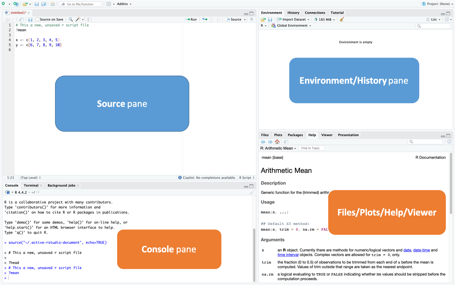
Shortcut to run code: Place cursor on a line → Ctrl + Enter (Windows) or Cmd + Enter (Mac)
One Critical RStudio Setting
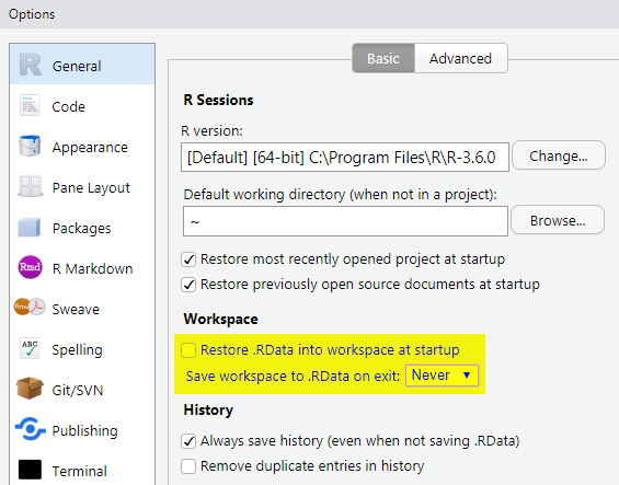
Before doing anything else, apply these settings for reproducibility:
Tools > Global Options > General > Basic
Uncheck “Restore .RData into workspace at startup”
Set “Save workspace to .RData on exit” → Never
This ensures a clean, reproducible workspace every session.
Getting Set Up: RStudio Projects
A Project keeps all your files (data, scripts, figures) in one folder and sets the working directory automatically.
Create a new project:
Click the blue cube (top-right) → New Project
Choose New Directory > New Project
Name it (e.g., Basic-R-Training) and choose a location
Click Create Project
Recommended folder structure:
Basic-R-Training/
├── data/         # Raw and cleaned datasets
├── scripts/      # R analysis scripts
├── figures/      # Saved plots
└── documents/    # Notes, reports
Key Benefits of RStudio Projects:
Automatically sets your working directory to your project folder
Makes file paths simple and relative (e.g., "data/my_data.csv").
Enhances reproducibility and collaboration.
R Basics: Objects in R
R is an object-oriented language. This means everything you create and manipulate in R—like numbers, text, datasets, and plots—is considered an object.
During an R session, objects are created and stored by name.
Results of calculations can be stored in objects using the assignment operators:
An arrow (<-) formed by a less than character and a hyphen without a space!. In RStudio (Alt + -)
Use summary() to see basic statistics for each variables
Subsetting
Using iris data, a built-in data frame with 150 rows and 5 columns.
Code
iris # the whole data frame iris[1, 1] # 1st element in 1st column iris[1, 6] # 1st element in the 6th column iris[, 1] # first column in the data frame iris[1] # first column in the data frame iris[1:3, 3] iris[3, ] # the 3rd row iris[1:6, ] # the 1st to 6th rowsiris[c(1,4), ] # rows 1 and 4 only iris[c(1,4), c(1,3) ] iris[, -1] # the whole except first columniris$Sepal.Length # Also extracts a column 'Sepal.Length'iris[,c("Sepal.Width", "Petal.Width")]# extract by name of column
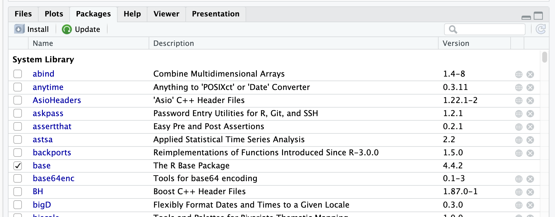
Installing and Loading Packages
Packages are collections of R functions, data, and compiled code in a well-defined format.
There are three categories of packages.
1. Base Packages: Providing the basic functionality, maintained by the R Core Development group. Currently, there are 14 packages, these are
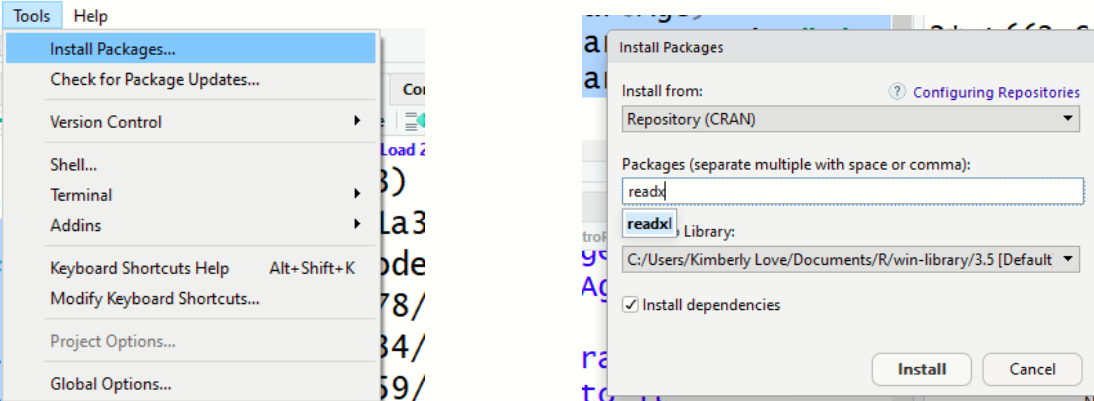
Installing a package is a one-time setup to download it onto your computer.
Loading a package with library() is required in each new R session to use its functions.
Code
# LOAD (do this every time you start a new script)library(tidyverse)library(readxl)library(writexl)library(labelled)
Note
If you get an error like "there is no package called 'dplyr'", you need to install it first
Installation downloads the package; loading makes it available for use
Only need to install once, but must load in every new session or script
Getting Help
Code
?read_csv # Help page for a functionhelp("lm") # Alternative syntax??survival # Search across all installed packages
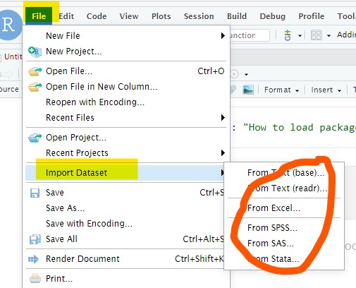
Reading and Writing data
Importing data is rather easy in R but that may also depend on the nature of the data to be imported and from what format.
Most data are in tabular form such as a spreadsheet or a comma-separated file (.csv).
Base R has a series of read functions to import tabular data from plain text files with columns delimited by: space, tab, and comma, with or without a header containing the column names.
With an added package it is also possible to import directly from a Microsoft Excel spreadsheet format or other foreign formats from various sources.
Importing from local files
In base R the standard commands to read text files are based on the read.table()function.
The following table lists the collection of the base R read functions.
For more details use the help command help(read.table) that will display help for all.
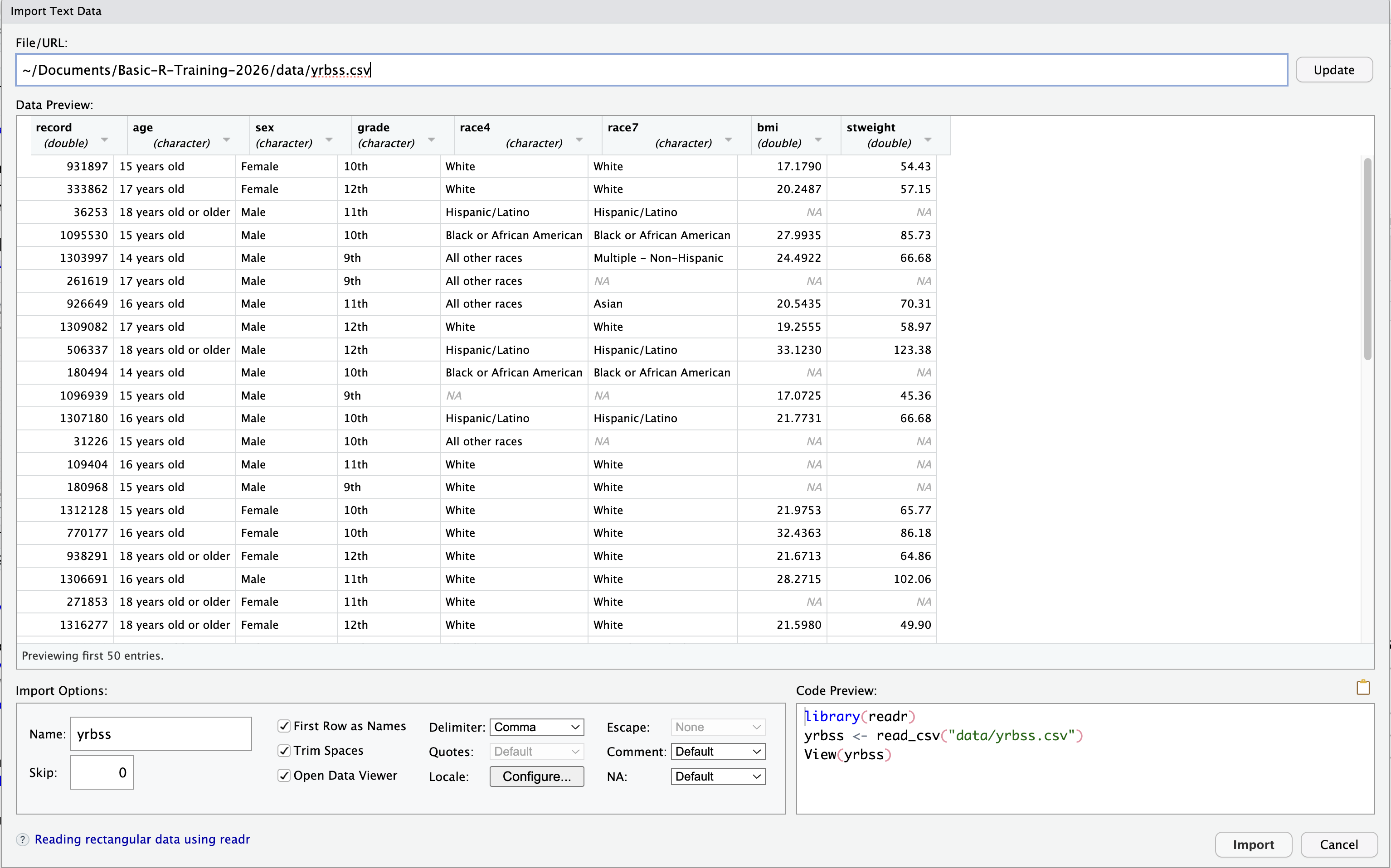
The data import wizard is a quick and easy way to import your data
Inside the data wizard, you can copy the code from the code-preview window, then paste the code into the code chunk of your r script or quarto document.
Composing the data import code…
Writing the import data function can be tricky. Try the import wizard pictured above. THEN, paste the code from the Code Preview section into your script.
Easily write import data function
Exporting Data
R to csv: Use readr package
Code
library(readr)write_csv(data, "data/mydata.csv")
R to a text file:
Code
write.table(data, "mydata.txt", sep="\t")
R to Excel: The readxl package is for reading Excel files only. For writing to Excel, the writexl package is a great modern and simple option.