Univariate Time Series Analysis with R

Leykun Getaneh (MSc)

NDMC, EPHI

November 17 - 21, 2025

🎯 Session Objectives

By the end of this session, you will be able to:

• Understand core concepts of univariate time series: trend, seasonality, stationarity
• Load, explore, and visualize time series data in R
• Perform decomposition and stationarity diagnostics
• Build, tune, and evaluate ARIMA/SARIMA models
• Generate and evaluate forecasts with confidence intervals

Notes:

• This session assumes you are comfortable with basic R and tidyverse.
• We’ll use a monthly malaria cases dataset for hands-on practice.

📈 Time Series Foundations

What is a Time Series?

• A time series is a sequence of data points collected at successive, equally spaced points in time.

• Our goal is often to understand past patterns or to forecast future values.

• Forecasting uses historical patterns to predict future values

• Application areas:

  • Public health (disease forecasting, demand for vaccines)
  • Economics/finance (inflation, sales, stock indices)
  • Energy (load forecasting), climate (temperature, rainfall), operations (inventory)

Key Components

• Trend (T): The long-term direction (up, down, or flat).
• Seasonal (S): A repeating, periodic pattern (e.g., monthly, quarterly).
• Cyclical (C): Long-term patterns not tied to a specific calendar period (e.g., business cycles). We often group this with Trend.
• Residual/Noise (R): The random, irregular component left over.

Setup and Data

# Core packages
library(tidyverse)
library(lubridate)

# Time series packages
library(forecast)   # ARIMA, auto.arima, forecast, ggtsdisplay
library(tseries)    # adf.test
library(urca)       # KPSS (ur.kpss)
library(zoo)        # zoo objects
library(xts)        # xts objects

# Visualization
library(scales)

Read and inspect the data

malaria_data <- read_csv("data/malaria_regx.csv")

glimpse(malaria_data)

Rows: 96
Columns: 4
$ year        <dbl> 2016, 2016, 2016, 2016, 2016, 2016, 2016, 2016, 2016, 2016…
$ month       <chr> "January", "February", "March", "April", "May", "June", "J…
$ total_cases <dbl> 32047, 26018, 33362, 24993, 45026, 68702, 44575, 37700, 59…
$ date        <date> 2016-01-01, 2016-02-01, 2016-03-01, 2016-04-01, 2016-05-0…

# Basic checks and ordering by date
malaria <- malaria_data |>
  mutate(date = as.Date(date)) |>
  arrange(date) |>
  mutate(month = factor(month, levels = month.name, ordered = TRUE))
# Quick head
head(malaria)

# A tibble: 6 × 4
   year month    total_cases date      
  <dbl> <ord>          <dbl> <date>    
1  2016 January        32047 2016-01-01
2  2016 February       26018 2016-02-01
3  2016 March          33362 2016-03-01
4  2016 April          24993 2016-04-01
5  2016 May            45026 2016-05-01
6  2016 June           68702 2016-06-01

Notes:

• Columns: year, month, total_cases, date (monthly start dates).
• We standardize month ordering for consistent plotting.

Visual Inspection

Before modeling, always visualize the raw data to identify obvious patterns.

malaria |>
  ggplot(aes(x = date, y = total_cases)) +
  geom_line(color = "steelblue", linewidth = 0.9) +
  geom_point(color = "steelblue", size = 0.6) +
  labs(title = "Monthly Malaria Cases (2016-2023)",
       x = "Date", y = "Total cases (monthly)") +
  theme_minimal(base_size = 14)

Exercise 1: Visual Inspection

• Look at the plot on the previous slide.
• Discuss with a partner:
  1. Do you see a trend? (Is it generally increasing or decreasing?)
  2. Do you see seasonality? (Is there a repeating pattern within each year?)

📦 Handling Time Series Data

Time Series Objects in R

• ts: The classic base R time series object. Required for the forecast package.
• zoo / xts: Robust options for irregular time series or finance.
• tsibble: Modern “tidy” time series frames (used with fable).

For this module, we focus on ts objects for ARIMA modeling.

Creating a ts Object

• Use ts() for the forecast package functions like auto.arima.

# We need:
# 1. The data vector ($total_cases)
# 2. The start date (Year, Month)
# 3. The frequency (12 for monthly)
malaria_ts <- ts(malaria_data$total_cases, 
                 start = c(2016, 1), 
                 frequency = 12)

# Plot it with the generic `autoplot`
autoplot(malaria_ts) +
  geom_line(color = "steelblue", linewidth = 0.7) +
  labs(title = "Malaria Cases as a 'ts' Object") +
  theme_minimal()

Seasonal plot to inspect monthly patterns

# Seasonal plot to inspect monthly patterns
library(forecast)
ggseasonplot(malaria_ts, linewidth = 0.7) + 
    scale_y_continuous(labels = label_number(scale_cut = cut_short_scale())) +
  labs(title = "Seasonal Plot of Malaria Cases") +
  theme_minimal()

🔍 Diagnostics & Decomposition

What is Decomposition?

• Decomposition means splitting the time series into its components: \(Y(t) = Trend(t) + Seasonal(t) + Residual(t)\) (Additive)

  \(Y(t) = Trend(t) \times Seasonal(t) \times Residual(t)\) (Multiplicative)

• Additive: Use when the seasonal variation is roughly constant.

• Multiplicative: Use when seasonal variation increases as the trend increases. (Ours looks multiplicative!)

Decomposition with stl()

We’ll use stl() (Seasonal and Trend decomposition using Loess), which is robust. We apply it to our ts object.

# STL Decomposition
decomp <- stl(malaria_ts, s.window = "periodic")
autoplot(decomp) + theme_minimal()

What Is Stationarity?

• A stationary series is one whose statistical properties (mean, variance, covariance) do not change over time.

• It has no trend and no changing seasonality.

• Why care? Most time series models (like ARIMA) assume the data is stationary.

• How? We often difference the data (e.g., \(Y_t - Y_{t-1}\)) to make it stationary. This is the “I” (for Integrated) in ARIMA.

• Types:

  • Strict (all moments invariant) vs. weak/second-order (mean/variance/ACF invariant)
  • Trend-stationary (deterministic trend removable) vs. difference-stationary (unit root)

Exercise:

• Inspect the malaria plot: does level or variance change over time? What transformation might help?

Checking for Stationarity: ACF/PACF

• ACF (Autocorrelation Function): Measures the correlation between \(Y_t\) and \(Y_{t-k}\) (past values).
• PACF (Partial Autocorrelation Function): Measures the correlation between \(Y_t\) and \(Y_{t-k}\) after removing the effects of the lags in between.

. . .

ACF/PACF Rules of Thumb:

• Non-stationary (Trend): ACF plot shows a very slow, linear decay.
• Seasonal: ACF plot shows strong spikes at the seasonal lags (12, 24, 36…).
• Stationary AR(p): ACF decays, PACF cuts off after lag p.
• Stationary MA(q): ACF cuts off after lag q, PACF decays.

ACF/PACF Plots in R

# Create training and test sets
# Training: 2016-2022 (7 years, 84 obs)
# Test: 2023 (1 year, 12 obs)
train_ts <- window(malaria_ts, end = c(2022, 12))
test_ts <- window(malaria_ts, start = c(2023, 1))

Let’s look at the ACF for our training data.

# We use ggAcf and ggPacf from the 'forecast' package
ggAcf(train_ts, lag.max = 36) +
  labs(title = "ACF for Malaria Training Cases") + theme_bw()

• Observation: Very slow decay and strong spikes at 12, 24, 36. This data is not stationary and is seasonal.

Stationarity Tests

• We use statistical tests to be more formal.
• ADF (Augmented Dickey-Fuller) Test:
  • \(H_0\) (Null): The series is non-stationary (has a unit root).
  • \(H_a\) (Alternative): The series is stationary.
  • Goal: We want a small p-value (< 0.05) to reject \(H_0\) and conclude the series is stationary.

. . .

library(tseries) # For adf.test

# Run ADF test on the training data
adf.test(train_ts)

    Augmented Dickey-Fuller Test

data:  train_ts
Dickey-Fuller = -2.3861, Lag order = 4, p-value = 0.4175
alternative hypothesis: stationary

• Result: The p-value is large (e.g., > 0.1), so we fail to reject \(H_0\). We conclude the data is non-stationary (as we saw in the plot).

Differencing

# Create a first-differenced series:
train_ts_diff1 = diff(train_ts, lag = 1)

# create a seasonal differenced series
train_ts_seas_diff <- diff(train_ts, lag = 12)

# create combined differences (non seasonal and seasonal differencing)
train_ts_comb_diff <- diff(diff(train_ts, lag = 12))

# 2. Plot the differenced data:
autoplot(train_ts_comb_diff) + 
    labs(title = "First differenced Series") + 
  theme_minimal()

# 3.Run the `adf.test()` on `diff_train_ts`.
adf.test(train_ts_comb_diff)

    Augmented Dickey-Fuller Test

data:  train_ts_comb_diff
Dickey-Fuller = -3.9024, Lag order = 4, p-value = 0.01914
alternative hypothesis: stationary

Visualizing ACF/PACF

# Correlation plots for the differenced (stationary) data
ggAcf(train_ts_comb_diff, lag.max = 48) + ggtitle("ACF (Non Seasonal & Seasonal Differenced)") + theme_minimal()
ggPacf(train_ts_comb_diff, lag.max = 48) + ggtitle("PACF (Non Seasonal & Seasonal Differenced)") + theme_minimal()

ARIMA Modeling

What is ARIMA?

ARIMA (Autoregressive Integrated Moving Average) is a popular statistical method used for analyzing and forecasting time series data. It predicts future points in a series by relying on its own past values, errors, and trends.

ARIMA(p, d, q) combines three key components to model:

• AR (p): Autoregressive part

  • \(X_t\) is a weighted sum of p past values.
  • “The value today is a function of yesterday’s value.”

• I (d): Integrated part

  • d is the number of differences needed to make the series stationary.
  • “We model the change from yesterday, not the raw value.”

• MA (q): Moving Average part

  • \(X_t\) is a weighted sum of q past forecast errors.
  • “The value today is a function of yesterday’s error.”

For a stationary series (after appropriate differencing), we typically model it with ARMA/ARIMA.

What is SARIMA?

SARIMA = Seasonal ARIMA. It adds seasonal components.

SARIMA(p, d, q) (P, D, Q)[s]

• (p, d, q): The non-seasonal parts (from the previous slide).
• (P, D, Q): The seasonal AR, I, and MA parts.
• [s]: The seasonal period (s=4,12, etc for us).

Manually finding these 6 numbers is not easy!

ARMA and SARMA Equations

For a stationary series (\(X_t\)) (after differencing), an ARMA((p,q)) model is

\[ X_t = \phi_1 X_{t-1} + \phi_2 X_{t-2} + \cdots + \phi_p X_{t-p} + \varepsilon_t + \theta_1 \varepsilon_{t-1} + \cdots + \theta_q \varepsilon_{t-q}, \]

or more compactly with the backshift operator (B):

\[ \phi(B) X_t = \theta(B)\varepsilon_t. \]

Where:

• \(X_t\): observed time series at time \(t\).
• \(\varepsilon_t\): white noise error term at time \(t\), usually \(\varepsilon_t \sim \text{i.i.d. }(0,\sigma^2)\).
• \(\phi_1, \dots, \phi_p\): nonseasonal AR parameters.
• \(\theta_1, \dots, \theta_q\): nonseasonal MA parameters.
• \(\phi(B) = 1 - \phi_1 B - \cdots - \phi_p B^p\): non-seasonal AR operator
• \(\theta(B) = 1 + \theta_1 B + \cdots + \theta_q B^q\): non-seasonal MA operator
• \(B\): backshift (lag) operator, \(B X_t = X_{t-1}\).
• \(p\) and \(q\): order of nonseasonal AR and MA components, respectively.

SARIMA Model Equation

SARIMA(p, d, q)(P, D, Q)[s] model:

\[ \Phi(B^s)\phi(B)(1 - B)^d (1 - B^s)^D X_t = \Theta(B^s)\theta(B)\varepsilon_t \]

Where:

• \(\phi(B) = 1 - \phi_1 B - \cdots - \phi_p B^p\): non-seasonal AR
• \(\theta(B) = 1 + \theta_1 B + \cdots + \theta_q B^q\): non-seasonal MA
• \(\Phi(B^s) = 1 - \Phi_1 B^s - \cdots - \Phi_P B^{Ps}\): seasonal AR
• \(\Theta(B^s) = 1 + \Theta_1 B^s + \cdots + \Theta_Q B^{Qs}\): seasonal MA
• \((1-B)^d\): differencing
• \((1-B^s)^D\): seasonal differencing
• \(s\): seasonal period (e.g., 12 for months)
• \(X_t\): observed time series at time \(t\).
• \(\varepsilon_t\): white noise error term at time \(t\), usually \(\varepsilon_t \sim \text{i.i.d. }(0,\sigma^2)\).
• \(B\): backshift (lag) operator, \(B X_t = X_{t-1}\).
• \(s\): seasonal period (e.g., \(s = 12\) for monthly data).
• \(d\): order of nonseasonal differencing.
• \(D\): order of seasonal differencing.
• \(P\) and \(Q\): order of seasonal AR and MA components, respectively.
• \(\Phi_1, \dots, \Phi_P\): seasonal AR parameters.
• \(\Theta_1, \dots, \Theta_Q\): seasonal MA parameters.
• Sometimes a constant or drift term is included (handled via include.constant or include.drift in forecast::Arima).

ACF/PACF Patterns for ARMA Models

(for stationary series, after appropriate differencing)

Model	ACF behavior	PACF behavior
AR(p)	Tails off	Cuts off after lag (p)
MA(q)	Cuts off after lag (q)	Tails off
ARMA(p,q)	Tails off	Tails off

Notes:

• “Cuts off” = near-zero after that lag.
  
• “Tails off” = decays gradually, often geometrically or in a damped pattern.
  
• Use these patterns on the differenced (stationary) series to guide choice of (p) and (q).

4. Building ARIMA/SARIMA Model

We’ll fit the model to our training data (train_ts).

• Use auto.arima() for a strong baseline; validate via residual diagnostics and Ljung–

• Forecast with intervals; compare models by AIC, BIC, and AICc and accuracy

# Create training and test sets: last 12 months as test
# Training: 2016-2022 (7 years, 84 obs)
# Test: 2023 (1 year, 12 obs)
train_ts <- window(malaria_ts, end = c(2022, 12))
test_ts <- window(malaria_ts, start = c(2023, 1))

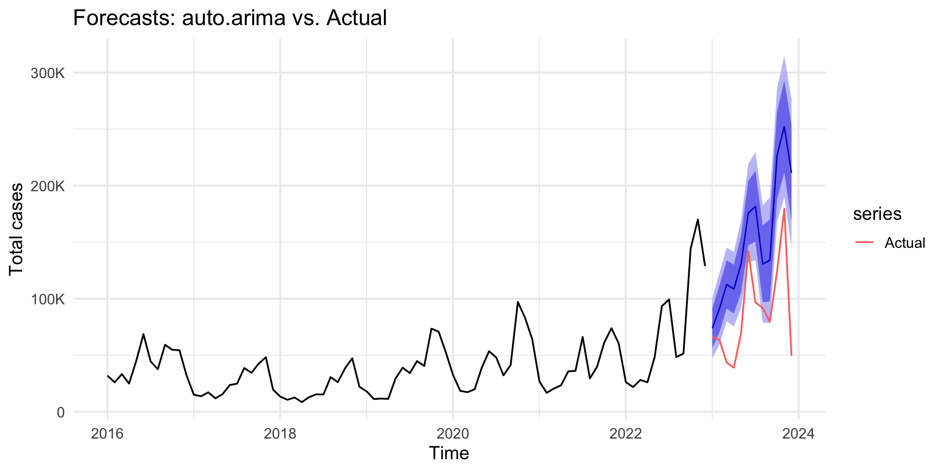
# Find the best ARIMA model automatically
library(forecast)
fit_auto <- auto.arima(
  train_ts,
  seasonal = TRUE,
  stepwise = FALSE, approximation = FALSE
)
fit_auto

Series: train_ts 
ARIMA(0,1,4)(0,1,0)[12] 

Coefficients:
          ma1      ma2      ma3     ma4
      -0.3639  -0.3532  -0.0978  0.5622
s.e.   0.1179   0.1354   0.1091  0.1326

sigma^2 = 186134492:  log likelihood = -775.65
AIC=1561.3   AICc=1562.22   BIC=1572.61

Manual SARIMA modeling

# Example manual model: seasonal difference often D=1 for monthly
# Use ACF/PACF patterns to pick p,q,P,Q; here we try SARIMA(4,1,3)(0,1,0)[12]
fit_manual <- forecast::Arima(train_ts,
                              order = c(4,1,3),
                              seasonal = c(0,1,0),
                              include.constant = FALSE)
fit_manual

Series: train_ts 
ARIMA(4,1,3)(0,1,0)[12] 

Coefficients:
         ar1      ar2      ar3     ar4      ma1     ma2     ma3
      0.6400  -0.3002  -0.1301  0.3982  -1.0385  0.2852  0.1229
s.e.  0.3524   0.3780   0.2890  0.1529   0.3701  0.5246  0.3102

sigma^2 = 193247818:  log likelihood = -775.3
AIC=1566.6   AICc=1568.92   BIC=1584.7

tibble(
  model = c("ARIMA(0,1,4)(0,1,0)[12]", "manual SARIMA(4,1,3)(0,1,0)[12]"),
  AIC  = c(fit_auto$aic, fit_manual$aic),
  BIC = c(fit_auto$bic, fit_manual$bic),
  AICc = c(fit_auto$aicc, fit_manual$aicc)
) |> 
  arrange(AIC)

# A tibble: 2 × 4
  model                             AIC   BIC  AICc
  <chr>                           <dbl> <dbl> <dbl>
1 ARIMA(0,1,4)(0,1,0)[12]         1561. 1573. 1562.
2 manual SARIMA(4,1,3)(0,1,0)[12] 1567. 1585. 1569.

Based on the above results, the ARIMA(0,1,4)(0,1,0)[12] model has the smallest selection criteria and is therefore the preferred model.

🔍 Check Residuals

• After fitting, we must check the residuals.
• Good residuals should look like white noise:
  1. Mean of zero.
  2. No significant autocorrelation (all ACF spikes are inside the blue lines).
  3. Normally distributed.
• checkresiduals() runs all these diagnostics for us!

# Plot diagnostics for model residuals
checkresiduals(fit_auto) 

    Ljung-Box test

data:  Residuals from ARIMA(0,1,4)(0,1,0)[12]
Q* = 9.232, df = 13, p-value = 0.7552

Model df: 4.   Total lags used: 17

• Ljung-Box Test:
  • \(H_0\): The residuals are independently distributed (no autocorrelation).
  • Goal: We want a large p-value (> 0.05) to fail to reject \(H_0\).
• Observation: If the p-value is large and the ACF plot looks good, our model is likely adequate.

Forecasting

Forecasting and Forecast comparison

fc_auto <- forecast::forecast(fit_auto, h = 12)
fc_manual <- forecast::forecast(fit_manual, h = 12)

autoplot(fc_auto) +
  autolayer(test_ts, series = "Actual") +
  labs(title = "Forecasts: auto.arima vs. Actual",
       y = "Total cases") +
  scale_y_continuous(labels = label_number(scale_cut = cut_short_scale())) +
  theme_minimal(base_size = 14)

5. Forecast Evaluation and Confidence Intervals

• How good was our forecast? We can compare our forecast to the test_ts data we held back.

• Evaluate on holdout: MAE, RMSE, MAPE

• accuracy() gives us common error metrics

acc_auto <- accuracy(fc_auto, test_ts) |> as_tibble() |> mutate(model = "auto.arima")
acc_manual <- accuracy(fc_manual, test_ts) |> as_tibble() |> mutate(model = "manual")

bind_rows(acc_auto, acc_manual) |>
  select(model, ME, MAE, RMSE, MAPE, MASE, ACF1) |>
  arrange(RMSE)

# A tibble: 4 × 7
  model           ME    MAE   RMSE  MAPE  MASE    ACF1
  <chr>        <dbl>  <dbl>  <dbl> <dbl> <dbl>   <dbl>
1 manual       1517.  8518. 12134.  25.6 0.563 -0.0187
2 auto.arima   1583.  8509. 12185.  26.5 0.562 -0.0256
3 auto.arima -65309. 65309. 75796.  95.8 4.31   0.109 
4 manual     -73249. 73249. 84795. 109.  4.84   0.142 

Final Forecast

Forecasting the Actual Future

1. Our model (fit_auto) was built only on the training set.
2. We validated it on the test set.
3. Now, to forecast the real future, we should re-fit the model on ALL available data (malaria_ts).

# Example solution for the wrap-up exercise:
fit_best <- forecast::auto.arima(malaria_ts, stepwise = FALSE, approximation = FALSE)
fc_best <- forecast::forecast(fit_best, h = 12)

autoplot(fc_best) +
  labs(title = "12-Month Forecast on full series",
       y = "Total cases") +
  scale_y_continuous(labels = label_number(scale_cut = cut_short_scale())) +
  theme_minimal(base_size = 14)

Final Forecast

fit_best

Series: malaria_ts 
ARIMA(0,1,1)(0,1,1)[12] 

Coefficients:
          ma1     sma1
      -0.5697  -0.2810
s.e.   0.1234   0.1498

sigma^2 = 380100453:  log likelihood = -937.32
AIC=1880.64   AICc=1880.95   BIC=1887.9

Session Summary

• We learned to plot time series with ggplot2 and forecast::autoplot.
• We used ts objects.
• We decomposed a series with stl() and checked stationarity with adf.test() and ggAcf().
• We built a SARIMA model automatically using auto.arima().
• We checked model quality with checkresiduals().
• We generated and evaluated forecasts using forecast() and accuracy().

Extensions

• ETS (Error, Trend, Seasonal): Exponential smoothing models (often comparable to ARIMA).

• Prophet (Meta): Handles multiple seasonalities and holidays well; robust to outliers.

• ARIMAX/SARIMAX (ARIMA with exogenous variables)

• Machine Learning/ Deep Learning: RNNs (LSTM/GRU/TFT), XGBoost

Capstone Exercise: HDSS Mortality Forecasting

Using your HDSS site data, Build a valid ARIMA/SARIMA model to predict mortality trends for the upcoming year to support health intervention planning?

References

• Shumway & Stoffer (2017). Time Series Analysis and Its Applications with R Examples.

• Montgomery, C. L., Jennings, M. K., & Kulahci, M. (2015). Introduction Time Series Analysis and Forecasting, New Jersey: John Willey & Sons.

• Hyndman, Athanasopoulos (2021). Forecasting: Principles and Practice (3rd ed.). https://otexts.com/fpp3/